“Eras” of Transformers
Processing an entire Numerai era at once with Transformers.
Just give me the code 🛠️:
GPU -> Run all notebook that generates a submission file. Runs within 15 mins. Another notebook is at the end that helps with deployment to compute-lite.
Update (23-Nov-2023): Updated the code with sliding window attention so now you can use vanilla attention
If you are new to Numer.ai’s tournaments, following posts might be helpful to get context about this post.
- https://docs.numer.ai/tournament/learn
- An easy guide to “The hardest tournament on the planet”
- Let’s talk about Signals
Might not be accurate. But still worth a try… looking at everything (all) at once!
The Data (Eras) ⌗
The provided data set (v4.1: Sunshine) contains obfuscated stock market data of past decades divided into groups called “Era” (an integer number). Eras represents a relative sense of timing, meaning era 1 happened before era 2 and so on until about 1050 eras in total. They are split into training and validation sets.
Era as a Sequence ⠿
Most models treat each row as a sample without any context of era. Approaches such as Era Boosting trains additional trees on the eras where the current ensemble is struggling. However, this still doesn’t look at the entire era for prediction. Since the primary goal of the data scientists is to rank the samples in a given era, it makes sense to be able to look at not only features but also all the samples in an era. This leads us to wondering what can we possibly perform if we can look at all the samples in an era and infer something from that! Possibilities are Era Clustering, Synthetic era generation in one pass, etc. The question is, can it provide some insights on movements of a group of stocks as it can see everything (all) at once?
I have been trying to work on these ideas for a while now. Initial experiments with LSTM didn’t succeed (maybe I couldn’t implement it properly back then). My initial trials with Transformers treated each row as as a sequence by using embedding of 5 unique input values {0, 1, 2, 3, 4}. However, It should be able to process entire era at once, simply by Transposing.
The (Era)Transformer to the rescue 🤖
Instead of treating each row as a sample, the era is padded to a fixed MAX_LENGTH and thus is treated as a sequence. The selected features are fed as embedding to the model along with mask at padded locations as shown in the illustration below.

# caching

def pad_sequence(inputs, padding_value=-1, max_len=None):
    if max_len is None:
        max_len = max([input.shape[0] for input in inputs])
    padded_inputs = []
    masks = []
    for input in inputs:
        pad_len = max_len - input.shape[0]
        padded_input = F.pad(input, (0, 0, 0, pad_len), value=padding_value)
        mask = torch.ones((input.shape[0], 1), dtype=torch.float)
        masks.append(
            torch.cat((mask, torch.zeros((pad_len, 1), dtype=torch.float)), dim=0)
        )
        padded_inputs.append(padded_input)
    return torch.stack(padded_inputs), torch.stack(masks)

def convert_to_torch(era, data):

    inputs = torch.from_numpy(
                data[feature_names].values.astype(np.int8))
    labels = torch.from_numpy(
                data[target_names].values.astype(np.float32))

    padded_inputs, masks_inputs = pad_sequence(
            [inputs], padding_value=PADDING_VALUE, max_len=MAX_LEN)
    padded_labels, masks_labels = pad_sequence(
            [labels], padding_value=PADDING_VALUE, max_len=MAX_LEN)

    return {
        era: (
            padded_inputs,
            padded_labels,
            masks_inputs
        )
    }

def get_era2data(df):
    res = Parallel(n_jobs=-1, prefer="threads")(
        delayed(convert_to_torch)(era, data)
        for era, data in tqdm(df.groupby("era_int")))
    era2data = {}
    for r in tqdm(res):
        era2data.update(r)
    return era2data

era2data_train = get_era2data(train)
era2data_validation = get_era2data(validation)
class TransformerEncoder(nn.Module):
def __init__(
self,
input_dim,
d_model,
output_dim,
num_heads,
num_layers,
dropout_prob=0.15,
max_len=5000,
):
super(TransformerEncoder, self).__init__()
self.input_dim = input_dim
self.output_dim = output_dim
self.num_heads = num_heads
self.num_layers = num_layers
self.dropout_prob = dropout_prob
self.d_model = d_model
self.positional_encoding = PositionalEncoding(d_model, max_len)
self.fc = nn.Sequential(
nn.Linear(d_model, d_model),
)
# Encoder layers
self.layers = nn.ModuleList(
[
nn.Sequential(
MultiHeadModularAttention(
d_model, num_heads, attention_type="vanilla"
), # multi-head attention
nn.LayerNorm(d_model), # layer normalization
FeedForwardLayer(
d_model=d_model
), # mixture of experts
nn.Dropout(dropout_prob), # dropout
)
for _ in range(num_layers)
]
)
self.mapper = nn.Sequential(
nn.Linear(input_dim, d_model), nn.Linear(d_model, d_model)
)
def forward(self, inputs, mask=None):
x = self.mapper(inputs)
# Add positional encoding; not needed in this case; doesn't hurt either
x = x + self.positional_encoding(x)
# Apply encoder layers
for layer in self.layers:
layer_output = layer[0](x, mask)
for sublayer in layer[1:]:
layer_output = sublayer(layer_output)
x = x + layer_output
return xThe positional encoding is added to the input. However, as we don’t know how the samples are even ranked originally, it might not be very helpful to use it but adding it wouldn’t hurt. The next step was to get the attention mechanism working.
The vanilla attention was too heavy for my laptop GPU so I tried using something like a Linear Attention as it would reduce the matrix multiplication load to first D_MODEL and then MAX_LEN. The standard Colab runtime in the provided notebook uses the vanilla attention mechanism on the provided small subset of features as it has higher GPU memory. The notebook has both available as a drop-in replacement for Multi-head attention block. Use whichever works for you.
Results
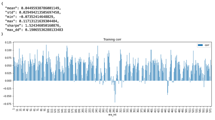
The experiments in the provided Colab uses “small” feature subset due to memory limitations. However, it uses the vanilla attention mechanism. Below is a small model trained on small feature set for 10 iterations on low learning rate to optimize for MSE and Pearson’s correlation.
A loss function that would enforce orthogonal embeddings in the encoder output would make much more sense for clustering. The current implementation is more of an early experiment and will get more accurate to perfect implementation. It seem to be working though.
Training Performance
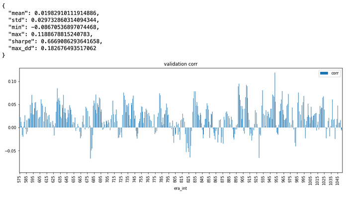
Validation Performance
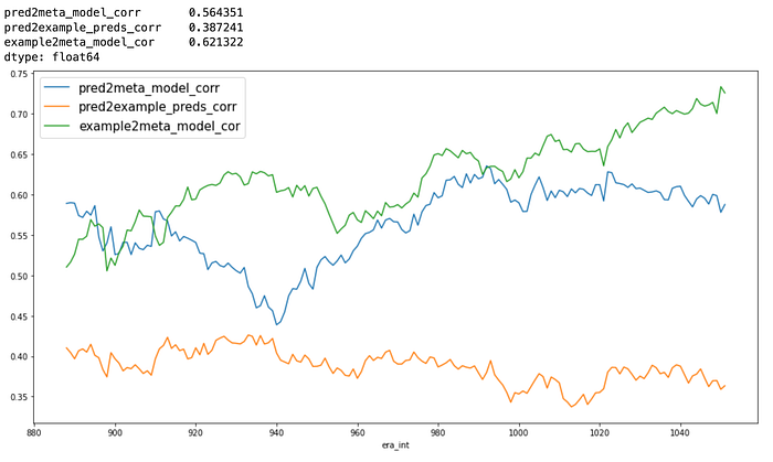
Relative to meta-model and example_model predictions
- “pred” is the trained model;
- “meta_model”: provided historical meta model predictions;
- “example”: provided example model predictions
The predictions are not highly correlated to the meta-model and the example_predictions. Not necessarily, but a unique loss function may help in improving True Contribution (TC) performance. This needs to be validated by live performance though.
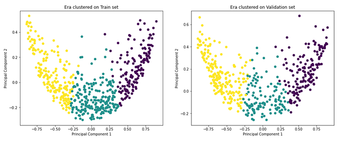
Clustering
What’s Next?
- Run Colab notebook (GPU->Run all). Generates a submission file
- Expand the feature set (small -> medium -> full set)
- Play with Attention mechanisms.
- Loss functions to get better embeddings 📉
- We have full idea of data in Signals; It will be much more applicable there.
- Generate synthetic Eras using Diffusion process
- Self-supervised training
- Randomize target weights. May their contribution be with us. (just need to un-comment)
BibTeX
@article{surajpnumeraitransformers,
  author={Suraj Parmar},
  title={"Eras" of Transformers},
  year={2023},
  url={https://parmarsuraj99.medium.com/era-of-transformers-792e5960e287},
}
References
- https://github.com/lucidrains/linear-attention-transformer
- https://numer.ai/data/v4.1
- Again Colab notebook
- ChatGPT + Github Copilot 👽
